Merging Data in a Spreadsheet
This is a really useful set of spreadsheet skills to be able to do. Partly it's here because it's tricky to find in the other place I put it on the web. Mainly it's here because I told MJ I'd put it here for her!
The situation is that you have data in two separate spreadsheet tables. The tables must have some shared data, but there's also data you need to get from one table into the other. But there's not necessarily any obvious order to the data - and there may even be some data in one table that's not in the other (and vice versa).
So, for example:
- A list of students with their UPN in one table but without names. The second table has their UPN and their name
- A list of countries of the world with development indicators - but some countries are missing from the second table - so it's hard to simple sort them alphabetically.
The example I'm going to work through is the second one - because I have the screenshots already done. It also doesn't involve putting kids names up on the internet...
Let's get ready to Merge (data)
Here's what to do: (NB: this is quite tricky. Some serious geek involved)
1. Get the two sets of data open in the two spreadsheets. Delete any columns you know you don't need. The key is that you need to have one piece of data in both sheets (the UPN or the country name). This data item wants to be unique to each row (or as close to unique as possible - it will work with names but it really needs to be the full name).
2. Copy the "second" set of data into the first sheet - leaving a few columns gap between the two sets of data (on my screenshot I have one column blank - this isn't really enough). I'll assume that you want to add something from the "second" set to the "first" set - so that the student name is in the second set and you want to add it to the first set.
3. Make sure that the unique data item (the UPN or the country name) is the first column in the second set of data. If necessary copy and paste the column of data. This is really important - it won't work otherwise!
4. Highlight the data you just pasted in - all of it (but not any blank rows underneath). Now you need to define a name for this data (Windows: Formulas > Define name; Mac: Insert > Name). I called my dataset dataB; you can call it anything you want but you cannot use spaces (names, student_names, dave, cookies - whatever).
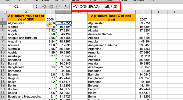
5. Then, in the cell at the end of the first set of data, put a formula along the lines of =VLOOKUP(A2, dataB, 2, 0). Check the screenshot to see what I did here - and check below to see how you'll need to change your formula...

My formula looks at whatever is in cell A2 up in the range of items called dataB. It then pastes into the cell the formula is in the item from the second column (the 2) in dataB. And the last 0 isn't doing anything directly but is massively important.
You will need to change the cells and so on:
- A2 is the cell you want to use in the first set of data (to the left of where you're entering the formula). It might be the cell the UPN is in - it does not need to be the first column in this table
- dataB is whatever you've called the data range you copied in (names, cookies etc...)
- 2 is the column number that you want to take the data out of in the named range. I wanted to take the data out of the second column in dataB so I have a 2. If the name of the child is in the fourth column then you'd have a 4, for example
- you just need the 0 at the end. Trust me. I'm a doctor (not) (there are reasons for this...)
You're not done yet - keep going!
6. Copy this formula all the way down the column. You may find you get some #N/A items. This is OK - it's because your formula couldn't find the unique data item from that row in the second data table.
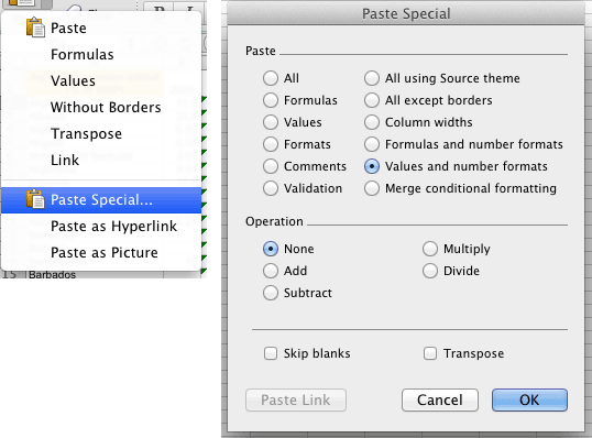
7. Highlight all the looked up items. Copy them, move to the next column and Paste Special - using the Values option (or Values and number formats if it's numerical data perhaps).
To Paste Special use the Home tab on the ribbon and click the little arrow next to the Paste button on the left. Both Windows and Mac versions of Excel should be OK from here - choose the Values format...

This is super important to do - you want the values rather than the formulas as otherwise when you delete the second data table you'll lose the values you just merged in.
8. Delete the column you put the VLOOKUP function in. You can also delete the second data table, for example.
And there you go - sets of data merged.
Final notes
As I said up top, this is a little tricky but the geek points you can score with it can be awesome. I originally wrote this up on the old SLN geography forum - hence the screenshot using development indicators. It should work for most versions of Excel and possibly, in similar ways, for other spreadsheet software.
Feel free to ask for help. I'd appreciate any feedback on the clarity (or lack of) of these instructions.
There are, of course, almost certainly better ways to do this. There's probably a database function of some kind which will do the job better and more easily. Or maybe an array function. Or maybe it would be easier to build a nice little relational database. But, y'know, sometimes a nice, straightforward (well...) spreadsheet function is actually easier in the long run.
